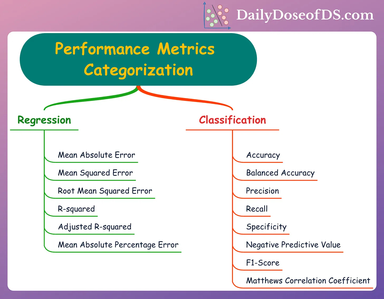
evaluation metrics for classification and regression

Performance metrics are used to assess the performance of a model on a given dataset.

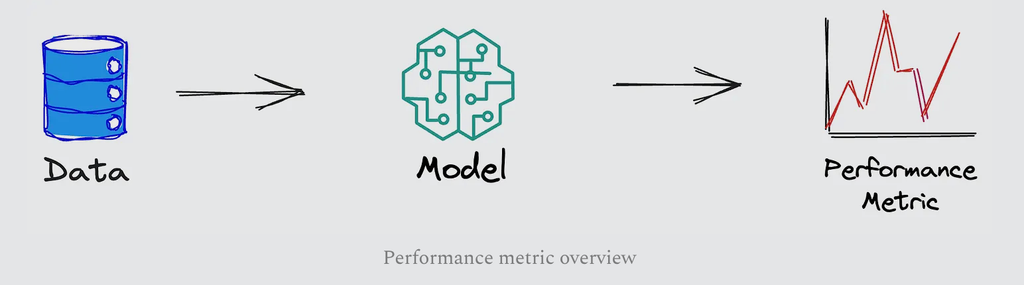
1. Performance Metrics for Regression

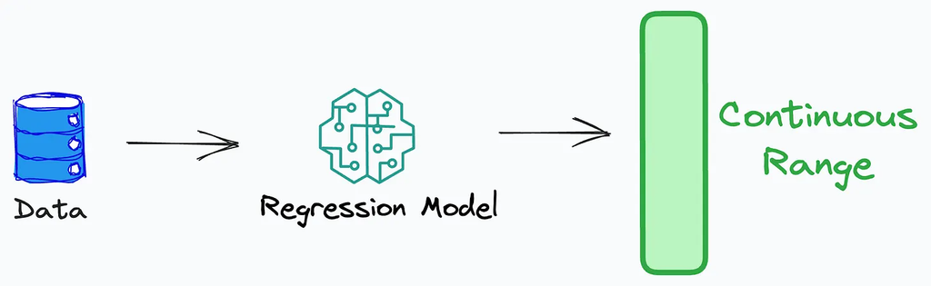
Regression metrics measure how close predictions are to actual numeric values. The exact choice depends on whether you care more about absolute error, large outliers, or error in the original unit.

Mean Absolute Error (MAE)

What is it?

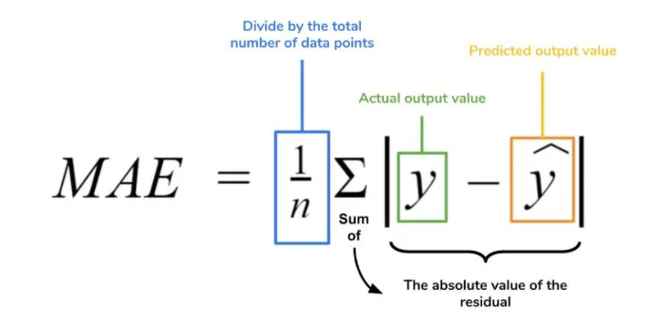
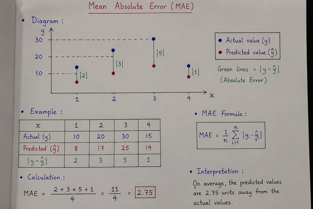
Mean Absolute Error measures the average magnitude of errors between predicted and actual values, without considering their direction. It’s the simplest metric to understand.

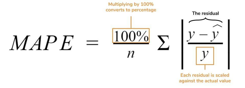
Where: n is the number of data points; y is the actual value; y_hat is the predicted value.

Code Example


import numpy as np

def calculate_mae(y_true, y_pred):
    return np.mean(np.abs(y_true - y_pred))

# Example
actual = [10, 15, 12, 8, 14]
predicted = [8, 14, 11, 9, 15]

mae = calculate_mae(np.array(actual), np.array(predicted))
print(f"MAE: {mae}")

Output: MAE: 1.4

When to use it?

When you need a metric that’s easy to understand and explain
When all errors should be treated equally
When you’re less concerned about outliers
When the error magnitude is directly interpretable in your domain

Real-world example

For house price predictions, an MAE of $10,000 means that, on average, our predictions are off by $10,000. This straightforward interpretation makes it valuable for communicating with non-technical stakeholders.

Mean Squared Error (MSE)

What is it?

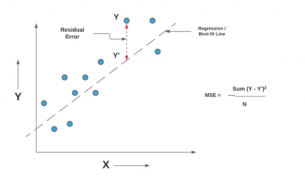
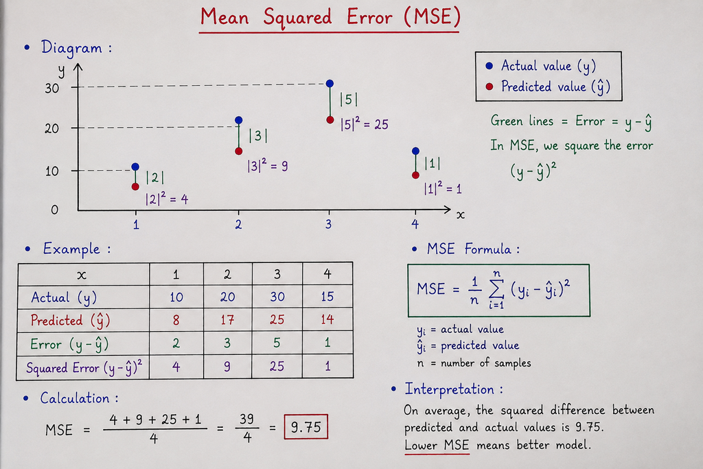
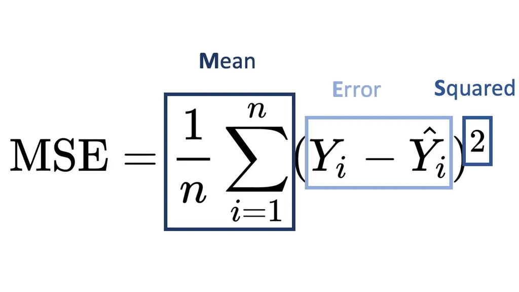
Mean Squared Error calculates the average of squared differences between predicted and actual values. By squaring the errors, it penalises larger errors more heavily than smaller ones.

Code Example


def calculate_mse(y_true, y_pred):
    return np.mean((y_true - y_pred) ** 2)

mse = calculate_mse(np.array(actual), np.array(predicted))
print(f"MSE: {mse}")  # Output: MSE: 2.2

Output: MSE: 2.2

When to use it?

When you want to penalize larger errors more than smaller ones
When outliers should have a bigger impact on your model evaluation
When the dataset has no extreme outliers that would overly distort the metric
When computational efficiency is important

Real-world example

In weather forecasting, predicting a temperature 10°F off is much worse than being 2°F off. MSE would penalise the 10°F error 25 times more than the 2°F error (100 vs. 4), appropriately reflecting the greater impact of larger prediction errors.

Mean Squared Error chart — Mean Squared Error for a regression problem

Root Mean Squared Error (RMSE)

What is it?

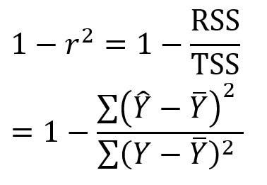
Root Mean Squared Error is simply the square root of MSE. Like MSE, it penalises larger errors more than smaller ones, but it brings the error measurement back to the original units of the target variable.

Code Example


def calculate_rmse(y_true, y_pred):
    return np.sqrt(np.mean((y_true - y_pred) ** 2))

rmse = calculate_rmse(np.array(actual), np.array(predicted))
print(f"RMSE: {rmse}")  # Output: RMSE: 1.483

Output: RMSE: 1.483

When to use it?

When you want errors in the same unit as the target variable
When you need a metric that penalizes large errors more than small ones
When comparing models with different target scales
When outliers are important to consider but should not dominate completely

Real-world example

In pharmaceutical dosage prediction, an RMSE of 5mg means the model’s predictions have an average error magnitude of 5mg, with larger errors contributing more to this figure. This is crucial because even small overdoses can be harmful.

Mean Absolute Percentage Error (MAPE)

What is it?

Mean Absolute Percentage Error measures the average percentage difference between predicted and actual values. It shows how far the predictions are off in percentage terms.

Code Example


def calculate_mape(y_true, y_pred):
    return 100 * np.mean(np.abs((y_true - y_pred) / y_true))

# Avoid zeros in y_true when using this metric
actual_no_zeros = [10, 15, 12, 8, 14]
predicted = [8, 14, 11, 9, 15]

mape = calculate_mape(np.array(actual_no_zeros), np.array(predicted))
print(f"MAPE: {mape}%")  # Output: MAPE: 11.9%

Output: MAPE: 11.9%

Note: Avoid zeros in y_true when using MAPE.

When to use it?

When you want to express errors as percentages rather than absolute values
When comparing performance across different scales
When the relative error is more important than the absolute error
When your data doesn’t contain values close to or equal to zero

Real-world example

In retail sales forecasting, a MAPE of 15% means predictions are off by 15% on average. This information helps retailers understand forecast accuracy relative to actual sales volumes, which is more useful than absolute numbers when comparing across stores of different sizes.

R-squared (Coefficient of Determination)

What is it?

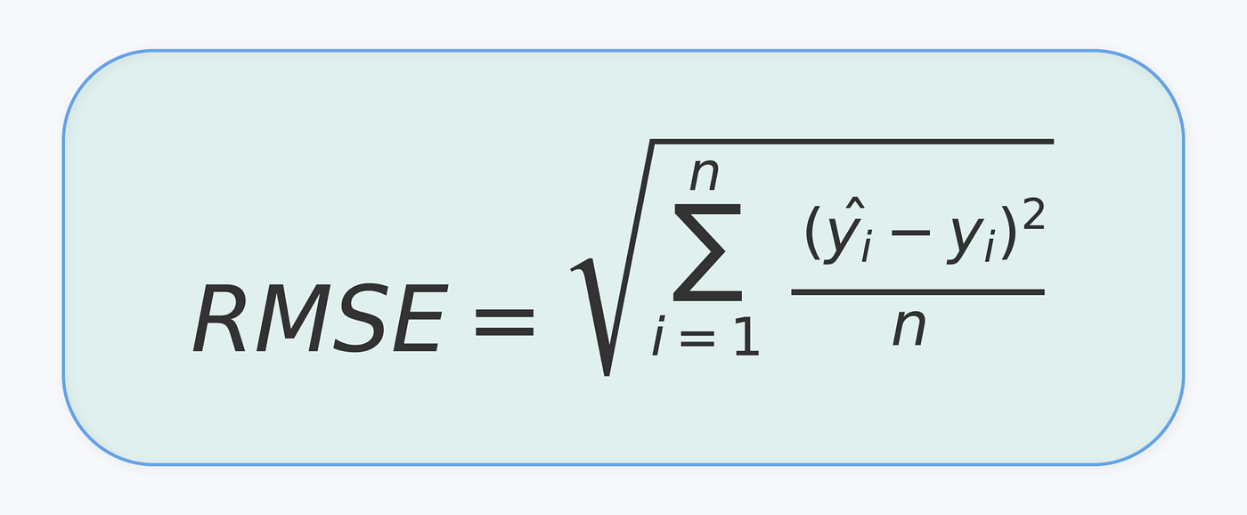
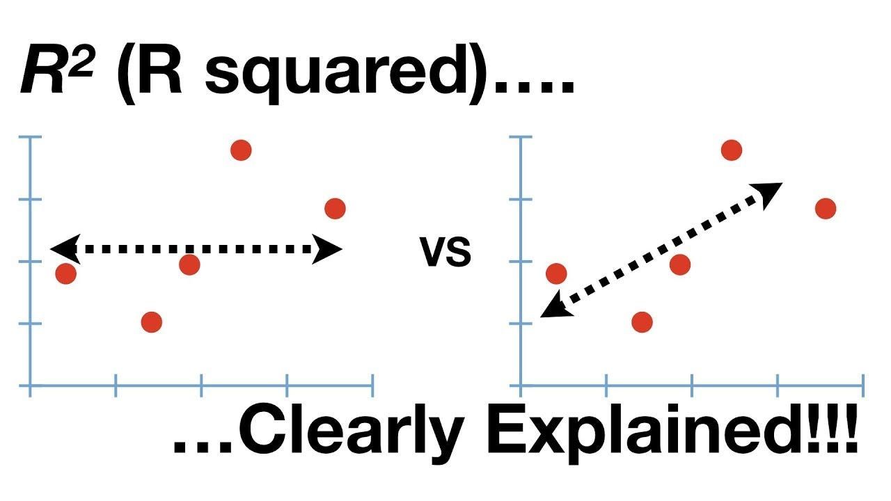
R-squared measures how well the model explains the variance in the target variable compared to simply using the mean. It ranges from 0 to 1, with 1 indicating that the model explains all the variability.

Code Example


def calculate_r2(y_true, y_pred):
    y_mean = np.mean(y_true)
    ss_total = np.sum((y_true - y_mean) ** 2)
    ss_residual = np.sum((y_true - y_pred) ** 2)
    return 1 - (ss_residual / ss_total)

r2 = calculate_r2(np.array(actual), np.array(predicted))
print(f"R-squared: {r2}")  # Output might be around 0.7-0.9

Output: R-squared: around 0.7-0.9

Note: Avoid zeros in y_true when using R-squared.

When to use it?

When you want to know how much variance your model explains
When comparing models on the same dataset
When you need a normalized metric between 0 and 1
When communicating with audiences familiar with statistical concepts

Real-world example

In credit risk modelling, an R-squared value of 0.75 means the model explains 75% of the variance in default risk based on the features used. This information helps financial institutions understand how complete their risk assessment model is.

Choosing the Right Metric

When selecting an evaluation metric for your regression model, consider these factors: 1. Business impact: Which type of errors are most costly in your domain? 2. Data characteristics: Does your data have outliers? Are all points equally important? 3. Interpretability needs: Who needs to understand the metric and make decisions based on it? 4. Comparison requirements: Are you comparing models with different features or scales?

Best practices:

Use multiple metrics to get a comprehensive view of model performance
Consider domain-specific requirements when prioritizing metrics
Be consistent with metrics when comparing different models
Communicate limitations of chosen metrics to stakeholders

Conclusion

Each metric offers distinct insights, yet no single metric provides a comprehensive picture. Understanding the strengths and weaknesses of each metric allows data scientists to make more informed decisions about model selection and improvement. By choosing appropriate evaluation metrics, you can ensure your regression models deliver real-world value and accurately solve the problems they’re designed to address.

What metrics do you typically use for regression problems? Do you prioritise certain metrics for specific applications? Share your experiences in the comments below!

2. Performance Metrics for Classification

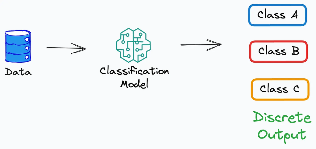
Classification models predict discrete labels rather than continuous values, so the emphasis shifts from distance to correctness, class balance, and the cost of specific mistakes.

Accuracy

Accuracy is the fraction of predictions that were correct.


def calculate_accuracy(y_true, y_pred):
    return np.mean(np.array(y_true) == np.array(y_pred))

Precision and Recall

Precision asks: of everything the model flagged as positive, how much was actually positive? Recall asks: of everything that was actually positive, how much did the model catch?


def calculate_precision_recall(y_true, y_pred):
    y_true, y_pred = np.array(y_true), np.array(y_pred)
    tp = np.sum((y_pred == 1) & (y_true == 1))
    fp = np.sum((y_pred == 1) & (y_true == 0))
    fn = np.sum((y_pred == 0) & (y_true == 1))

    precision = tp / (tp + fp) if (tp + fp) > 0 else 0
    recall = tp / (tp + fn) if (tp + fn) > 0 else 0
    return precision, recall

F1 Score

The F1 score balances precision and recall into a single number using their harmonic mean.


def calculate_f1(precision, recall):
    if precision + recall == 0:
        return 0
    return 2 * (precision * recall) / (precision + recall)

Confusion Matrix

Rather than collapsing performance into one number, a confusion matrix lays out every combination of predicted vs. actual class, making it easy to see exactly what kind of mistakes a model tends to make.


import matplotlib.pyplot as plt
import seaborn as sns
from sklearn.metrics import confusion_matrix

cm = confusion_matrix(y_true, y_pred)
sns.heatmap(cm, annot=True, fmt='g', cmap='Blues')
plt.xlabel('Predicted')
plt.ylabel('Actual')
plt.show()

Conclusion

Choosing an evaluation metric is part of defining the problem correctly. The right metric depends on the target type, the cost of mistakes, and how the result will be used. In practice, reporting more than one metric usually gives the clearest picture.